Big O Notation can feel like an intimidating topic for many beginners diving into algorithms and software development. It’s especially nerve-wracking when it comes up during a coding interview—a space where you want to showcase your expertise.
I recently faced a similar scenario while interviewing for a software engineering role. The technical challenge included live problem-solving, where I confidently arrived at the correct solution. However, when asked about the time complexity of my approach, I stumbled and relied on guesswork to explain the Big O function.
This experience was a wake-up call. It pushed me to revisit Big-O-Notation, a concept I’d first learned in college but had only a surface-level understanding of. If you’re a beginner or someone aiming to sharpen their skills for coding rounds, this post is for you. It’s designed to demystify Big O Notation and serve as a handy resource for future reference.
Big thanks to the inclusive programming community, especially resources like NeetCode, which make advanced topics accessible for everyone!
Table of Contents
What Is Big O Notation?
Big O Notation is a mathematical framework used to describe how an algorithm performs as the size of the input grows. It evaluates the time (or space) complexity, helping software engineers compare solutions based on efficiency.
In simpler terms, Big O helps you understand how an algorithm’s performance scales:
- O represents the operation or function.
- n represents the size of the input.
Why Does It Matter?
Understanding Big O is essential for coding interviews and real-world software development. Efficient algorithms save time and resources, ensuring scalable systems. Mastering this concept can set you apart as a thoughtful, knowledgeable developer.
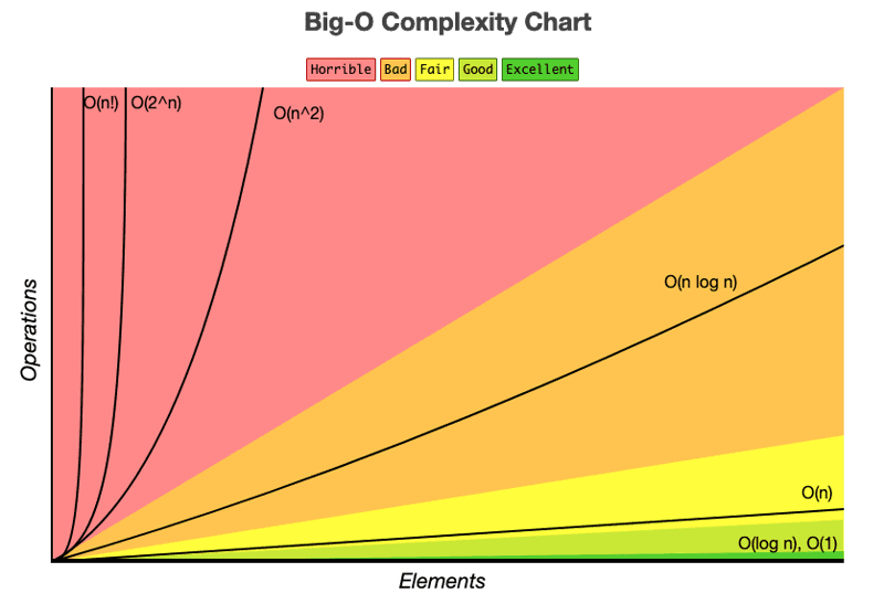
Let’s break down common Big O complexities with examples.
Common Big-O-Notations with Examples

O(1): Constant Time Complexity
When an algorithm’s execution time remains constant regardless of input size, it’s O(1). These are the fastest algorithms since they don’t depend on input size.
Example: Retrieving the first element of an array.
def first_element(arr):
    return arr[0]  # Always constant time, O(1)

n = [3, 1, 4, 1, 5]
print(first_element(n))  # Output: 3
O(n): Linear Time Complexity
In O(n), the execution time increases proportionally with the input size. If you need to iterate through every element, the time complexity is linear.
Example: Finding the maximum value in an unsorted array.
def find_max_value(arr):
    max_value = arr[0]
    for num in arr:
        if num > max_value:
            max_value = num
    return max_value

n = [3, 1, 4, 1, 5, 9, 2]
print(find_max_value(n))  # Output: 9
O(n²): Quadratic Time Complexity
O(n²) arises with nested loops, where each loop depends on the size of the input. This can quickly become inefficient for large datasets.
Example: Generating all combinations of two dice rolls.
def dice_combinations(sides):
    combinations = []
    for i in range(1, sides + 1):
        for j in range(1, sides + 1):
            combinations.append((i, j))
    return combinations

print(dice_combinations(6))  # Output: 36 combinations
O(log n): Logarithmic Time Complexity
Algos with O(log n) complexity become faster as input grows because they reduce the problem size with each iteration. These are common in divide-and-conquer approaches like binary search.
Example: Finding a value in a sorted array using binary search.
def binary_search(arr, target):
    left, right = 0, len(arr) - 1
    while left <= right:
        mid = (left + right) // 2
        if arr[mid] == target:
            return mid
        elif arr[mid] < target:
            left = mid + 1
        else:
            right = mid - 1
    return -1

sorted_array = [1, 2, 3, 4, 5, 6, 7, 8]
print(binary_search(sorted_array, 6))  # Output: 5
O(n log n): Linearithmic Time Complexity
Sorting algorithms like merge sort often fall under O(n log n). They divide the input (log n) and then perform linear work (n) to combine results.
Example: Sorting an array with merge sort.
def merge_sort(arr):
    if len(arr) <= 1:
        return arr
    mid = len(arr) // 2
    left = merge_sort(arr[:mid])
    right = merge_sort(arr[mid:])
    return merge(left, right)

def merge(left, right):
    result = []
    while left and right:
        result.append(left.pop(0) if left[0] < right[0] else right.pop(0))
    result.extend(left or right)
    return result

unsorted_array = [3, 1, 4, 1, 5, 9]
print(merge_sort(unsorted_array))  # Output: [1, 1, 3, 4, 5, 9]
O(2ⁿ): Exponential Time Complexity
When a function doubles its work with each additional input, it’s O(2ⁿ). Recursive problems without optimization often exhibit this complexity.
Example: Calculating Fibonacci numbers with naive recursion.
def fibonacci(n):
    if n <= 1:
        return n
    return fibonacci(n - 1) + fibonacci(n - 2)

print(fibonacci(5))  # Output: 5
Final Thoughts
Understanding Big O Notation is critical for building efficient, scalable algorithms and succeeding in coding interviews. As a beginner or seasoned developer, knowing how your code scales fosters better decision-making and robust software.

By grounding this knowledge in an inclusive programming community, you not only grow as an individual but also contribute to a shared pool of engineering excellence.
Keep practicing, keep learning, and remember: progress in coding is a marathon, not a sprint. Good luck on your journey! 🚀
Further Resources:


